Today, we're going to begin walking through the next sample experiment in Azure Machine Learning Studio, Sample 4: Cross Validation for Regression: Auto Imports Dataset. Let's start by looking at the experiment.
 |
| Sample 4: Cross Validation for Regression: Auto Imports Dataset |
We can see that this experiment is quite simple. We start by importing our data, imputing over the missing data and performing three different regressions. In this post, we'll focus on the initial data load and imputation. Let's begin by looking at the Automobile Price Data (Raw) visualization.
 |
| Automobile Price Data (Raw) (Visualization) 1 |
 |
| Automobile Price Data (Raw) (Visualization) 2 |
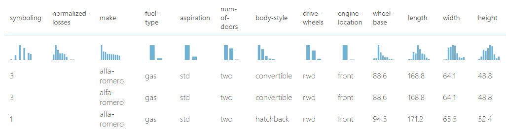
We can see that there are a number of different factors related to each vehicle, as well as the price of the vehicle. A very important question to ask of this data would be whether this price represents what someone actually paid or what the dealer is attempting to charge for it. The answer to this question would heavily influence the types of conclusions we could make about the data. Since this is a sample, we'll assume that "Price" represents how much someone actually paid for the vehicle.
Now, if the salesperson were able to accurately predict the price a customer would pay for the vehicle, then he or she could maximize his or her profit by selling for that amount. Conversely, if the customer were able to accurately predict the price another customer would pay for the vehicle, then he or she would know whether the current price is a good deal or not. Obviously, this type of information would be very beneficial for anyone who could create it. Let's see if we can do it!
Before we move on, we should note that we have no idea what the "Symboling" and "Normalized Losses" columns mean. In practice, we should never model with variables that we don't understand. So, we found this
snippet.
This data set consists of three types of entities: (a) the specification of an auto in terms of various characteristics, (b) its assigned insurance risk rating, (c) its normalized losses in use as compared to other cars.
The second rating corresponds to the degree to which the auto is more risky than its price indicates. Cars are initially assigned a risk factor symbol associated with its price. Then, if it is more risky (or less), this symbol is adjusted by moving it up (or down) the scale. Actuarians call this process "symboling". A value of +3 indicates that the auto is risky, -3 that it is probably pretty safe.
The third factor is the relative average loss payment per insured vehicle year. This value is normalized for all autos within a particular size classification (two-door small, station wagons, sports/speciality, etc...), and represents the average loss per car per year.
Let's look at the visualization for "Symboling".
 |
| Symboling (Statistics) |
 |
| Symboling (Histogram) |
The first thing we noticed is that getting a clean histogram using integers is virtually impossible. This is due to the fact that there are 5 spaces between the integers (3 - -2 = 5) but 6 unique values (-2, -1, 0, 1, 2, 3). Therefore, picking either one of these leads to either inaccurate bars where the final 2 integers are combined into a single bar (2 and 3, in this case) or confusing decimals on the axis.
 |
| Symboling (Histogram) (5 Bars) |
 |
| Symboling (Histogram) (6 Bars) |
In the end, we chose to go with a combination of these (5 + 6 = 11 Bars). This way, we can always tell exactly what values correspond to what integer, even if we have to do some light mental aerobics. Back on topic, we see that there are no automobiles in the "Safe" category (Symboling = -3). We also see that there are far more vehicles in the "Unsafe Range" (1 to 3) than there are in the "Safe Range" (-1 to -3). This is a pretty startling observation. However, our lack of expertise is making it very difficult to interpret these results. For now, we have to hold fast to our data science roots. If we don't know what it is, we shouldn't model with it. However, if we were experts in Automobile Insurance, we might be able to utilize these fields. In our case, we need to add a "Select Columns in Dataset" module to our experiment in order to remove these fields.
 |
| Select Columns in Dataset |
Next, let's look at the Clean Missing Data module.
 |
| Clean Missing Data |
We've talked about this module before in a previous
post. Basically, this tool will find any missing (or NULL) values in your dataset and replace them with another value of your choosing. In this case, we've chosen to replace missing values from all columns with 0. In the real world, this level of laziness could cause major problems with the analysis. So, what are the other options?
 |
| Cleaning Mode |
The formal name for this technique is
Imputation. There are a myriad of ways to deal with missing data. It primarily comes down to an important distinction. Is the missing data "Unknown" or "Non-existent"? For instance, if we built a table of Expenses by Month, it might look like this.
 |
| Expenses by Month |
We see that the value for March is missing. It could be that we did not have any expenses in March. In this case, the value for March is "Non-Existent" and should be replaced with 0. However, it could also be that we didn't keep track in March so we don't know what the value was. In this case, the value is "Unknown" and should be replaced with something other than 0.
As you can see, replacing "Non-Existent" values is simple. However, what are our options for replacing "Unknown" values? The most common method is to replace the missing values with a "common" value from the same column. The three prominent methods for defining "common" are Mean, Median and Mode. All three of these options are available within Azure ML. We prefer to use Median as it is less susceptible to outliers than Mean and a better indicator of "centrality" than Mode.
On the other hand, what if accuracy is a major concern and missing values are not acceptable? We have two options for that, removing the row or removing the column. If a particular set of rows has missing values across many columns, then it may be a good decision to remove those rows. Conversely, if many rows have missing values across a particular set of columns, then it may be a good decision to remove those columns. The decision of whether to remove rows, columns, or neither is based heavily on subject matter expertise. It is very easy to bias our dataset or lose valuable accuracy by removing too many rows or columns.
Finally, what if the previously described techniques are killing the accuracy of our model? Azure ML has two more advanced options for us,
MICE and
Probabilistic PCA. Instead of trying to explain these concepts ourselves, we'll pull from the
Azure documentation. Here's the description of MICE.
For each missing value, this option assigns a new value, which is calculated by using a method described in the statistical literature as Multivariate Imputation using Chained Equations or Multiple Imputation by Chained Equations.
In a multiple imputation method, each variable with missing data is modeled conditionally using the other variables in the data before filling in the missing values. In contrast, in a single imputation method (such as replacing a missing value with a column mean) a single pass is made over the data to determine the fill value.
All imputation methods introduce some error or bias, but multiple imputation better simulates the process generating the data and the probability distribution of the data.
For a general introduction to methods for handling missing values, see Missing Data: the state of the art. Schafer and Graham, 2002.
Here's the description of Probabilistic PCA.
Replaces the missing values by using a linear model that analyzes the correlations between the columns and estimates a low-dimensional approximation of the data, from which the full data is reconstructed. The underlying dimensionality reduction is a probabilistic form of Principal Component Analysis (PCA), and it implements a variant of the model proposed in the Journal of the Royal Statistical Society, Series B 21(3), 611–622 by Tipping and Bishop.
Compared to other options, such as Multiple Imputation using Chained Equations (MICE), this option has the advantage of not requiring the application of predictors for each column. Instead, it approximates the covariance for the full dataset. It may therefore offer better performance for datasets that have missing values in many columns.
The key limitations of this method are that it expands categorical columns into numerical indicators and computes a dense covariance matrix of the resulting data. It also is not optimized for sparse representations. For these reasons, datasets with large numbers of columns and/or large categorical domains (tens of thousands) are not supported due to prohibitive space consumption.
Simply put, if you have a large amount of missing data, you should consider using on of these techniques. Probabilistic PCA is better for dense, parametric datasets and MICE is better for sparse and/or non-parametric datasets.
With all of this in mind, let's look back at our data. In order to determine the best imputation, we'll use the "Summarize Data" module.
 |
| Summarize Data |
 |
| Summarize Data (Visualization) 1 |
 |
| Summarize Data (Visualization) 2 |
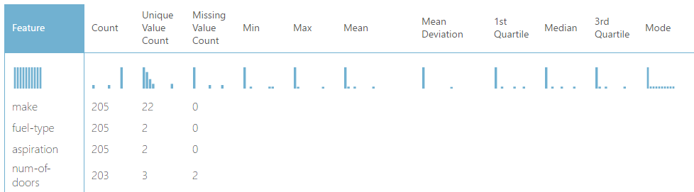
The visualization for the Summarize Data module gives us some summary statistics about each column, including how many missing values it has. The columns with missing values are shown in the preceding pictures. The first thing to note is that the "Price" column has 4 missing values. Since we are attempting to predict "Price", it would not be appropriate to impute values into that column. So, let's start by removing those 4 rows and see if we still have more missing values.
 |
| Remove Rows with Missing Price |
 |
| Remove Rows with Missing Price (Visualization) 1 |
 |
| Remove Rows with Missing Price (Visualization) 2 |
Removing those 4 rows definitely helped our Price. However, it didn't eliminate the missing values for the other columns. Next, let's look at the only string feature, "Num of Doors".
 |
| Num of Doors |
We can see that this column takes two values "two" and "four", with two rows having missing values. Unfortunately, most of the imputation algorithms built into Azure ML are designed to work with numeric data, not strings. We decided to test this just to see what would happen. The "Custom Substitution", "Remove Entire Row", "Remove Entire Column" and "Replace with Mode" options work exactly like we expected. However, the "Replace Using MICE" and "Replace Using Probabilistic PCA" successfully ran, but didn't do anything. Finally, the "Replace with Mean" and "Replace with Median" options failed to run at all. In our case, we have two options. We can either replace the Nulls with "Unknown" or replace them with the mode ("four"). We'll choose to use "Unknown" to minimize any possible bias.
As an interesting side note here, when we were using this example in a presentation, a knowledgeable car enthusiast suggested that we use the body type of the car to determine what we should replace these missing values with. This just goes to show that domain expertise can be very helpful when you are building data science solutions.
 |
| Replace Missing Num of Doors with Unknown |
 |
| Replace Missing Num of Doors with Unknown (Visualization) |
Next, we need to deal with the Numeric Variables. All of these represent legitimate numeric values that have only a few missing values. Therefore, it's not necessary to perform any of the complicated methodologies. In fact, we could simply remove these rows and be done with it. However, we don't know whether these rows contain valuable information for the regression. For now, we'll go with the "Replace with Median" option in order to reduce variability in the sample.
 |
| Replace Missing Numeric Values with Median |
One of the great things about Data Science is that there's always more to do. Did we use the "best" imputation method? Who knows. It all depends on what we're trying to get out of our model. In this case, it was simply exploratory and helped us learn so much about the different ways to clean some of our missing values. In fact, we could even use SQL, R or Python to create our own imputation algorithm inside a script. Stay tuned for the next post where we'll dig into linear regression. Thanks for reading. We hope you found this informative.
Brad Llewellyn
Data Scientist
Valorem
@BreakingBI
www.linkedin.com/in/bradllewellyn
llewellyn.wb@gmail.com


No comments:
Post a Comment